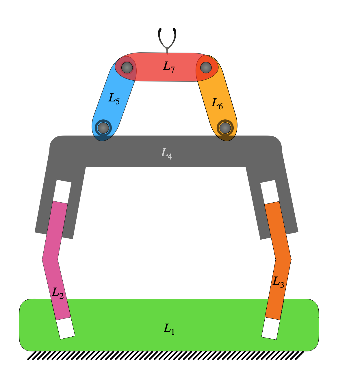
A figure of RRRRPPPP planar serial-parallel hybrid manipulator is shown
above. The corresponding adjacency matrix is given by
\[\begin{split}\bf{M} = \left[\begin{matrix}L_1 & P & P & O & O & O & O\\A & L_2 & O & P & O & O & O\\A & O & L_3 & P & O & O & O\\O & O & O & L_4 & R & R & O\\O & O & O & A & L_5 & O & R\\O & O & O & O & O & L_6 & R\\O & O & O & O & O & O & L_7\end{matrix}\right]\end{split}\]
Connecting paths:
All possible paths connecting the end-effector link from the base link,
are shown below.
\[\begin{split}\begin{matrix}
\text{Path 1:} \;\;\; L_1-L_2-L_4-L_5-L_7 \\
\text{Path 2:} \;\;\; L_1-L_3-L_4-L_5-L_7 \\
\text{Path 3:} \;\;\; L_1-L_2-L_4-L_6-L_7 \\
\text{Path 4:} \;\;\; L_1-L_3-L_4-L_6-L_7
\end{matrix}\end{split}\]
In order to check for possibility of redundant paths, the rank of the
connectivity matrix is considered.
\[\begin{split}\begin{matrix}
\bf{v}^{(1)}=\bf{V}_{(1,2)}+\bf{V}_{(2,4)}+\bf{V}_{(4,5)}+\bf{V}_{(5,7)} \\
\bf{v}^{(2)}=\bf{V}_{(1,3)}+\bf{V}_{(3,4)}+\bf{V}_{(4,5)}+\bf{V}_{(5,7)} \\
\bf{v}^{(3)}=\bf{V}_{(1,2)}+\bf{V}_{(2,4)}+\bf{V}_{(4,6)}+\bf{V}_{(6,7)} \\
\bf{v}^{(4)}=\bf{V}_{(1,3)}+\bf{V}_{(3,4)}+\bf{V}_{(4,6)}+\bf{V}_{(6,7)} \\
\end{matrix}\end{split}\]
\[\begin{split}\Rightarrow \begin{Bmatrix}
\bf{v}^{(1)} \\
\bf{v}^{(2)} \\
\bf{v}^{(3)} \\
\bf{v}^{(4)}
\end{Bmatrix} =
\begin{bmatrix}
1 & 1 & 1 & 1 & 0 & 0 & 0 & 0 \\
0 & 0 & 1 & 1 & 1 & 1 & 0 & 0 \\
1 & 1 & 0 & 0 & 0 & 0 & 1 & 1 \\
0 & 0 & 0 & 0 & 1 & 1 & 1 & 1
\end{bmatrix}
\begin{Bmatrix}
\bf{V}_{(1,2)} \\
\bf{V}_{(2,4)} \\
\bf{V}_{(4,5)} \\
\bf{V}_{(5,7)} \\
\bf{V}_{(1,3)} \\
\bf{V}_{(3,4)} \\
\bf{V}_{(4,6)} \\
\bf{V}_{(6,7)}
\end{Bmatrix}\end{split}\]
\[\Rightarrow \begin{Bmatrix}
\bf{v}^{(k)}
\end{Bmatrix} =
\begin{bmatrix}
\bf{C}_{\bf{V}}
\end{bmatrix}
\begin{Bmatrix}
\bf{V}_{(i,j)}
\end{Bmatrix}\]
Even though there are 4 equations, the rank of the matrix
\([\bf{C}_{\bf{V}}]\) is 3. This shows that only three independent
connecting paths from base to end-effector exist and hence one of the
paths should be redundant. The set of independent connecting paths can
be found by performing the row-reduced echelon form or the row echelon
form of \([\bf{C}_{\bf{V}}]^T\). The set of indices of pivot
columns indicates that the set of corresponding paths are independent.
By performing row-reduced echelon form on \([\bf{C}_{\bf{V}}]^T\),
the list of pivot columns is \((1,2,3)\), and hence the paths 1, 2
and 3 amount to a set of independent paths.
Now, given that the independent connecting paths are the first three
paths, the angular velocity connectivity matrix is considered as
follows.
\[\begin{split}\begin{matrix}
\bf{\omega}^{(1)}=\bf{\Omega}_{(1,2)}+\bf{\Omega}_{(2,4)}+\bf{\Omega}_{(4,5)}+\bf{\Omega}_{(5,7)} \\
\bf{\omega}^{(2)}=\bf{\Omega}_{(1,3)}+\bf{\Omega}_{(3,4)}+\bf{\Omega}_{(4,5)}+\bf{\Omega}_{(5,7)} \\
\bf{\omega}^{(3)}=\bf{\Omega}_{(1,2)}+\bf{\Omega}_{(2,4)}+\bf{\Omega}_{(4,6)}+\bf{\Omega}_{(6,7)}
\end{matrix}\end{split}\]
The \(\bf{\Omega}_{(i,j)}\) terms corresponding to prismatic
joints, i.e., \(\bf{\Omega_{(1,2)}}\),
\(\bf{\Omega_{(1,3)}}\), \(\bf{\Omega_{(2,4)}}\) and
\(\bf{\Omega_{(3,4)}}\) are set to zero. The equations would then
become
\[\begin{split}\begin{matrix}
\bf{\omega}^{(1)}=\bf{\Omega}_{(4,5)}+\bf{\Omega}_{(5,7)} \\
\bf{\omega}^{(2)}=\bf{\Omega}_{(4,5)}+\bf{\Omega}_{(5,7)} \\
\bf{\omega}^{(3)}=\bf{\Omega}_{(4,6)}+\bf{\Omega}_{(6,7)}
\end{matrix}\end{split}\]
\[\begin{split}\Rightarrow \begin{Bmatrix}
\bf{\omega}^{(1)} \\
\bf{\omega}^{(2)} \\
\bf{\omega}^{(3)}
\end{Bmatrix} =
\begin{bmatrix}
1 & 1 & 0 & 0 \\
1 & 1 & 0 & 0 \\
0 & 0 & 1 & 1
\end{bmatrix}
\begin{Bmatrix}
\bf{\Omega}_{(4,5)} \\
\bf{\Omega}_{(5,7)} \\
\bf{\Omega}_{(4,6)} \\
\bf{\Omega}_{(6,7)}
\end{Bmatrix}\end{split}\]
\[\Rightarrow \begin{Bmatrix}
\bf{\omega}^{(k)}
\end{Bmatrix} =
\begin{bmatrix}
\bf{C}_{\Omega}
\end{bmatrix}
\begin{Bmatrix}
\bf{\Omega}_{(i,j)}
\end{Bmatrix}\]
The rank of the matrix \([\bf{C_{\Omega}}]\) is 2, even though there
are three equations. Hence, only two independent equations exist. The
set of independent connecting paths can be found by performing
row-reduced echelon form or echelon form on \([\bf{C_{\Omega}}]^T\).
The set of indices of pivot columns would indicate the set of
corresponding independent paths in the context of angular velocity. By
performing row-reduced echelon form on \([\bf{C_{\Omega}}]^T\), the
list of pivoted columns is found to be (1,3), and hence the paths 1 and
3 amount to a set of independent paths in the context of angular
velocity.
Therefore, the independent linear velocities are \(\bf{v}^{(1)}\),
\(\bf{v}^{(2)}\) and \(\bf{v}^{(3)}\), and the independent
angular velocities are \(\bf{\omega}^{(1)}\) and
\(\bf{\omega}^{(3)}\).
\[\bf{v}^{(1)}=\dot{d}_{(1,2)} \bf{\hat{n}_{(1,2)}} + \dot{d}_{(2,4)} \bf{\hat{n}_{(2,4)}} + \dot{\theta}_{(4,5)} \bf{\hat{k}} \times \left( \bf{a} - \bf{r}_{(4,5)} \right) + \dot{\theta}_{(5,7)} \bf{\hat{k}} \times \left( \bf{a} - \bf{r}_{(5,7)} \right)\]
\[\bf{v}^{(2)}=\dot{d}_{(1,3)} \bf{\hat{n}}_{(1,3)} + \dot{d}_{(3,4)} \bf{\hat{n}}_{(3,4)} + \dot{\theta}_{(4,5)} \bf{\hat{k}} \times \left( \bf{a} - \bf{r}_{(4,5)} \right) + \dot{\theta}_{(5,7)} \bf{\hat{k}} \times \left( \bf{a} - \bf{r}_{(5,7)} \right)\]
\[\bf{v}^{(3)}=\dot{d}_{(1,2)} \bf{\hat{n}}_{(1,2)} + \dot{d}_{(2,4)} \bf{\hat{n}}_{(2,4)} + \dot{\theta}_{(4,6)} \bf{\hat{k}} \times \left( \bf{a} - \bf{r}_{(4,6)} \right) + \dot{\theta}_{(6,7)} \bf{\hat{k}} \times \left( \bf{a} - \bf{r}_{(6,7)} \right)\]
\[\bf{\omega}^{(1)} = \dot{\theta}_{(4,5)} \bf{\hat{k}} + \dot{\theta}_{(5,7)} \bf{\hat{k}}\]
\[\bf{\omega}^{(3)} = \dot{\theta}_{(4,6)} \bf{\hat{k}} + \dot{\theta}_{(6,7)} \bf{\hat{k}}\]
\[\begin{split}\begin{Bmatrix}\bf{v}^{(1)} \\ \bf{\omega}^{(1)}\end{Bmatrix} = \begin{Bmatrix}\bf{v} \\ \bf{\omega}\end{Bmatrix} = \left[\begin{matrix}- a_{y} + r_{(4,5)y} & n_{(1,2)x} & 0\\a_{x} - r_{(4,5)x} & n_{(1,2)y} & 0\\1 & 0 & 0\end{matrix}\right]\begin{Bmatrix}\dot{\theta}_{(4,5)}\\\dot{d}_{(1,2)}\\\dot{d}_{(1,3)}\end{Bmatrix} + \left[\begin{matrix}0 & - a_{y} + r_{(5,7)y} & 0 & n_{(2,4)x} & 0\\0 & a_{x} - r_{(5,7)x} & 0 & n_{(2,4)y} & 0\\0 & 1 & 0 & 0 & 0\end{matrix}\right]\begin{Bmatrix}\dot{\theta}_{(4,6)}\\\dot{\theta}_{(5,7)}\\\dot{\theta}_{(6,7)}\\\dot{d}_{(2,4)}\\\dot{d}_{(3,4)}\end{Bmatrix}\end{split}\]
Constraint equations:
\[\begin{split}\begin{Bmatrix}\bf{v}^{(2)}-\bf{v}^{(1)} \\ \bf{v}^{(3)}-\bf{v}^{(1)} \\ \bf{\omega}^{(3)}-\bf{\omega}^{(1)}\end{Bmatrix} = \bf{0}\end{split}\]
\[\begin{split}\Rightarrow \left[\begin{matrix}0 & - n_{(1,2)x} & n_{(1,3)x}\\0 & - n_{(1,2)y} & n_{(1,3)y}\\a_{y} - r_{(4,5)y} & 0 & 0\\- a_{x} + r_{(4,5)x} & 0 & 0\\-1 & 0 & 0\end{matrix}\right]\begin{Bmatrix}\dot{\theta}_{(4,5)}\\\dot{d}_{(1,2)}\\\dot{d}_{(1,3)}\end{Bmatrix} + \left[\begin{matrix}0 & 0 & 0 & - n_{(2,4)x} & n_{(3,4)x}\\0 & 0 & 0 & - n_{(2,4)y} & n_{(3,4)y} \\- a_{y} + r_{(4,6)y} & a_{y} - r_{(5,7)y} & - a_{y} + r_{(6,7)y} & 0 & 0 \\a_{x} - r_{(4,6)x} & - a_{x} + r_{(5,7)x} & a_{x} - r_{(6,7)x} & 0 & 0 \\1 & -1 & 1 & 0 & 0 \end{matrix}\right]\begin{Bmatrix}\dot{\theta}_{(4,6)}\\\dot{\theta}_{(5,7)}\\\dot{\theta}_{(6,7)}\\\dot{d}_{(2,4)}\\\dot{d}_{(3,4)}\end{Bmatrix}=\begin{Bmatrix} 0 \\ 0 \\ 0\end{Bmatrix}\end{split}\]
\[\begin{split}\bf{J_a} = \left[\begin{matrix}- a_{y} + r_{(4,5)y} & n_{(1,2)x} & 0\\a_{x} - r_{(4,5)x} & n_{(1,2)y} & 0\\1 & 0 & 0\end{matrix}\right]\end{split}\]
\[\begin{split}\bf{J_p} = \left[\begin{matrix}0 & - a_{y} + r_{(5,7)y} & 0 & n_{(2,4)x} & 0\\0 & a_{x} - r_{(5,7)x} & 0 & n_{(2,4)y} & 0\\0 & 1 & 0 & 0 & 0\end{matrix}\right]\end{split}\]
\[\begin{split}\bf{A_a} = \left[\begin{matrix}0 & - n_{(1,2)x} & n_{(1,3)x}\\0 & - n_{(1,2)y} & n_{(1,3)y}\\a_{y} - r_{(4,5)y} & 0 & 0\\- a_{x} + r_{(4,5)x} & 0 & 0\\-1 & 0 & 0\end{matrix}\right]\end{split}\]
\[\begin{split}\bf{A_p} = \left[\begin{matrix}0 & 0 & 0 & - n_{(2,4)x} & n_{(3,4)x} \\0 & 0 & 0 & - n_{(2,4)y} & n_{(3,4)y} \\- a_{y} + r_{(4,6)y} & a_{y} - r_{(5,7)y} & - a_{y} + r_{(6,7)y} & 0 & 0 \\a_{x} - r_{(4,6)x} & - a_{x} + r_{(5,7)x} & a_{x} - r_{(6,7)x} & 0 & 0 \\1 & -1 & 1 & 0 & 0 \end{matrix}\right]\end{split}\]
\[\bf{\widetilde{J}} = \bf{J_a}-\bf{J_p}\bf{A^{-1}_p}\bf{A_a}\]