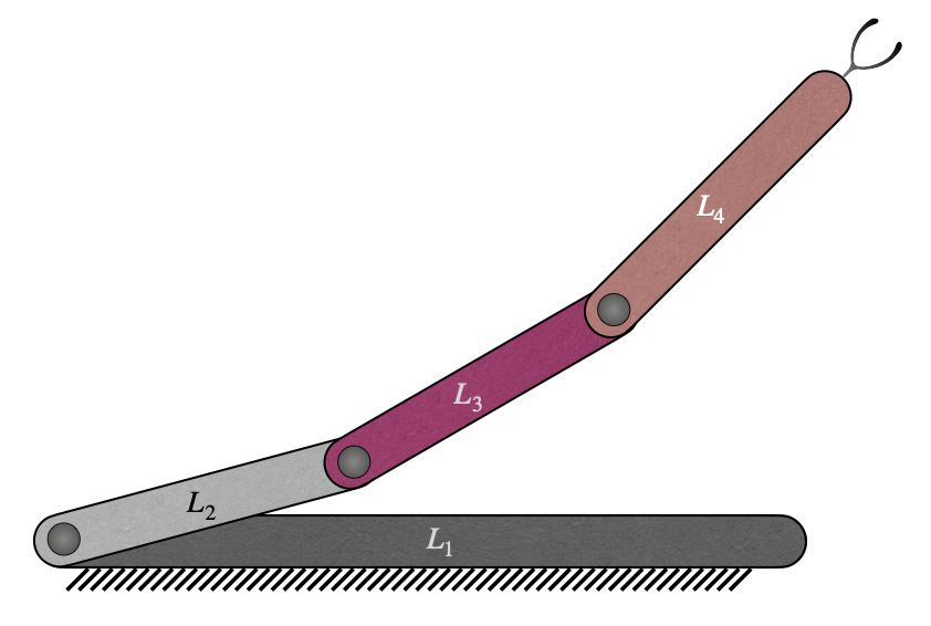
An RRR planar serial manipulator is considered as shown in the figure
above. The corresponding adjacency matrix is given by
\[\begin{split}\bf{M} = \left[\begin{matrix}L_1 & R & O & O \\A & L_2 & R & O\\O & A & L_3 & R\\O & O & A & L_4\end{matrix}\right]\end{split}\]
Connecting paths:
\[\text{Path 1:}\;\;\;\;L_1-L_2-L_3-L_4\]
Since this has only one connecting path, if the manipulator represented
by the matrix is valid then it must be a serial manipulator. Hence,
there would be only one independent set of formulation of linear and
angular velocities, and formulation of \([\bf{C}_{V}]\) and
\([\bf{C}_{\Omega}]\) are not required.
The following are the linear and angular velocity contributions to the
end-effector from each joint of the path, which are calculated by using
the formulation shown in table and by
using the convention that all the revolute joints of a planar
manipulator would have their axes on the xy-plane, thereby reducing the
unit vector along each axis to
\(\bf{\hat{n}}_{(i,j)}=\bf{\hat{k}}\), as mentioned in equation 20
of the main document.
\[\begin{split}\begin{matrix}
\bf{V_{12}}=\dot{\theta}_{(1,2)} \bf{\hat{n}_{(1,2)}} \times \left( \bf{a} - \bf{r}_{(1,2)} \right) = \dot{\theta}_{(1,2)} \bf{\hat{k}} \times \left( \bf{a} - \bf{r}_{(1,2)} \right) \\
\bf{V_{23}}=\dot{\theta}_{(2,3)} \bf{\hat{n}_{(2,3)}} \times \left( \bf{a} - \bf{r}_{(2,3)} \right) = \dot{\theta}_{(2,3)} \bf{\hat{k}} \times \left( \bf{a} - \bf{r}_{(2,3)} \right) \\
\bf{V_{34}}=\dot{\theta}_{(3,4)} \bf{\hat{n}_{(3,4)}} \times \left( \bf{a} - \bf{r}_{(3,4)} \right) = \dot{\theta}_{(3,4)} \bf{\hat{k}} \times \left( \bf{a} - \bf{r}_{(3,4)} \right)
\end{matrix}\end{split}\]
\[\begin{split}\begin{matrix}
\bf{\Omega_{12}}=\dot{\theta}_{(1,2)} \bf{\hat{n}_{(1,2)}} = \dot{\theta}_{(1,2)} \bf{\hat{k}} \\
\bf{\Omega_{23}}=\dot{\theta}_{(2,3)} \bf{\hat{n}_{(2,3)}} = \dot{\theta}_{(2,3)} \bf{\hat{k}} \\
\bf{\Omega_{34}}=\dot{\theta}_{(3,4)} \bf{\hat{n}_{(3,4)}} = \dot{\theta}_{(3,4)} \bf{\hat{k}}
\end{matrix}\end{split}\]
Therefore, the linear and angular velocities are given by the equations
below.
\[\bf{v}^{(1)}=\dot{\theta}_{(1,2)} \bf{\hat{k}} \times \left( \bf{a} - \bf{r}_{(1,2)} \right) + \dot{\theta}_{(2,3)} \bf{\hat{k}} \times \left( \bf{a} - \bf{r}_{(2,3)} \right) + \dot{\theta}_{(3,4)} \bf{\hat{k}} \times \left( \bf{a} - \bf{r}_{(3,4)} \right)\]
\[\bf{\omega}^{(1)}=\dot{\theta}_{(1,2)} \bf{\hat{k}} + \dot{\theta}_{(2,3)} \bf{\hat{k}} + \dot{\theta}_{(3,4)} \bf{\hat{k}}\]
Since this is a planar manipulator, the case of superfluous DOF does not
come into picture.
If the actuating joint velocities vector is considered to be
\(\bf{\Omega_a} = \{\dot{\theta}_{(1,2)} \; \dot{\theta}_{(2,3)} \; \dot{\theta}_{(3,4)}\}^T\),
the velocity of the end-effector is given by
\[\begin{split}\begin{Bmatrix}\bf{v} \\ \bf{\omega}\end{Bmatrix} = \begin{Bmatrix}\bf{v}^{(1)} \\ \bf{\omega}^{(1)}\end{Bmatrix} = \left[\begin{matrix}- a_{y} + r_{(1,2)y} & - a_{y} + r_{(2,3)y} & - a_{y} + r_{(3,4)y} \\a_{x} - r_{(1,2)x} & a_{x} - r_{(2,3)x} & a_{x} - r_{(3,4)x}\\1 & 1 & 1\end{matrix}\right]\begin{Bmatrix}\dot{\theta}_{(1,2)}\\\dot{\theta}_{(2,3)}\\\dot{\theta}_{(3,4)}\end{Bmatrix}\end{split}\]
\[\begin{split}\Rightarrow \begin{Bmatrix}\bf{v} \\ \bf{\omega}\end{Bmatrix} = \bf{J_a} \bf{\Omega_a}\end{split}\]
Therefore, the Jacobian of the manipulator is
\[\begin{split}\bf{\widetilde{J}} = \bf{J_a} = \left[\begin{matrix}- a_{y} + r_{(1,2)y} & - a_{y} + r_{(2,3)y} & - a_{y} + r_{(3,4)y}\\a_{x} - r_{(1,2)x} & a_{x} - r_{(2,3)x} & a_{x} - r_{(3,4)x}\\1 & 1 & 1\end{matrix}\right]\end{split}\]
Since it is a serial manipulator, the matrices \(\bf{J_p}\),
\(\bf{A_a}\) and \(\bf{A_p}\) do not come into picture.